Display Negative Numbers As Positive In Excel Chart
By leaving out the negative symbol Excel will display negative values as if they were positive values. You separate each segment with a semi-colon.

Best Excel Tutorial Chart With Negative Values
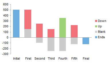
To recognize between positive and negative values well use color-coded stacked column.

Display negative numbers as positive in excel chart. If you are using earlier versions of Excel you can still create a Waterfall Chart using Stacked Column Chart. AVERAGEOFFSETB20COUNTB2N2-313 Creating an Excel moving average chart. When creating a pie chart the description of each section is called the category and the number connected to the category is called the value.
Click Kutools Charts Difference Comparison Column Chart with Percentage Change. A second IF function is then used to determine if the change from old to new is positive or negative. Hi quick question about number formatting for the axes.
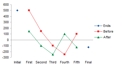
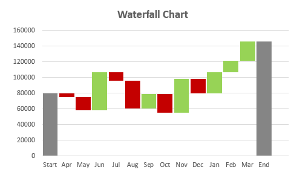
The base column will represent the starting point for the fall and rise of the chart. You will input all the negative numbers from the sales flow in the fall column and all the positive numbers in the rise column. A Bubble Chart in Excel is a relatively new type of XY Chart that uses a 3rd value besides the X and Y coordinates to define the size of the Bubble.
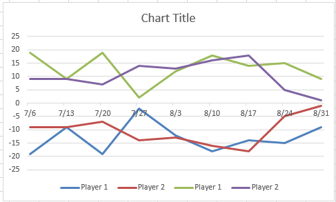
The negative differences are easy to see. The syntax of the TEXT function is as below. R-squared value Coefficient of Determination indicates how well the trendline corresponds to the data.
If you are displaying the positive and negative variances in separate series to display in different colors then you can add an additional column to calculate both the positive and negative variances. Insert three additional columns to your Excel table to represent the movement of the columns on the waterfall chart. Beginning with Excel 2013 the data labels for an XY or Bubble Chart series can be defined by simply selecting a range of cells that contain the labels whereas originally you had to link.
Follow our guide and you can build a great bridge chart in a few steps. Excel 2013 has a built-in feature that makes this process much easier. It is easy to format to show only thousands 123 but Id like to add the K symbol in case the number is 1000.
Additionally you can display the R-squared value. Or returns the smallest value in the arrayThe MIN. IFnew value old value0PN This IF statement returns a P for a positive change and an N for a negative change.
A negative value will display as its positive equivalent and a zero value simply wont appear. In the Percentage Change Chart dialog select the axis labels and series values as you need into two textboxes. Dont forget to separate each symbol with a semi-colon.
Creating a Waterfall Chart in Excel is an easy task if you have Microsoft Excel 2016 or a newer version. In the worksheet below we have outlined a single data seriesIf we had selected multiple series for the Pie Chart Excel would ignore all but the first. A Pie Chart displays one series of dataA data series is a row or column of numbers used for charting.
If both numbers are positive then the percentage change formula is used to display the result. The first segment applies to positive numbers the second to negative numbers the third to zero values and the fourth to text strings. On Format Cells under Number tab click Number in Category list then in Negative numbers list select number with bracketsThen click OK to confirm update.
If you are working with Excel 2010 or Excel 2013 we have good news for you. So one cell with number 123 will display 123 one cell with 123000 will show 123K. When I format my secondary axis I am trying to get the lowest negative numbers to disappear.
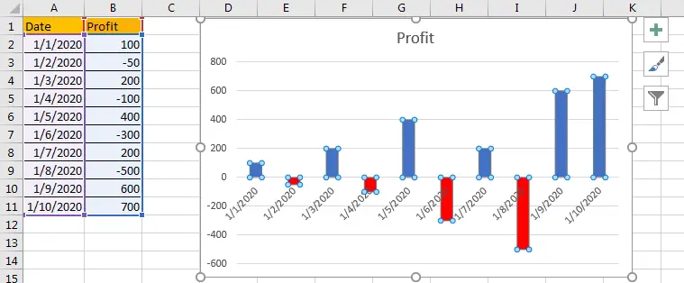
Most Excel users would be used to working with the concept of displaying negative numbers in a worksheet with a preceding sign in front of the number something a bit like this below where I have an example of monthly sales and the diference month on month of those sales figures. For example here is a format code that tells Excel to format positive numbers with no decimals and to enclose negative numbers with parentheses. Prepare a table contains some negative numbers.
Supposing B2 is the first number in the row and you want to include the last 3 numbers in the average the formula takes the following shape. Click Ok then dialog pops out to remind you a sheet will be created as well to place the data click Yes to continue. After free installing Kutools for Excel please do as below.
The first format in the string is normally for positive numbers but square brackets indicate a non-default condition for the first string. The range of the secondary axis is -3500 to 2000 and I want -500 to 2000 to be visible. How to display the trendline equation on a chart.
My data range includes both positive and negative numbers. Select the list contains negative numbers then right click to load menu. In MS Excel I would like to format a number in order to show only thousands and with K in from of it so the number 123000 will be displayed in the cell as 123K.
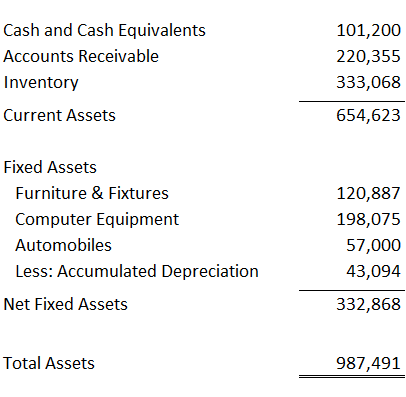
I want to display the total costs and credits per product however because all but 3 end up being a negative number they dont display in my pie chart only where SUM is positive. If you have already created a chart for your data adding a moving average trendline for that chart is a matter of seconds. Display Negative Numbers in Brackets.
When drawing the line of best fit in Excel you can display its equation in a chart. This means that any values less than 8 million will appear as the number of millions folloewd by capital M. The TEXT function is a build-in function in Microsoft Excel and it is categorized as a Text Function.
Click Format Cells on menu. Excel 2016 provides Waterfall Chart type. The semicolon with nothing following means that any other numbers will not be displayed.
TEXT value Format code Excel MIN function The Excel MIN function returns the smallest numeric value from the numbers that you provided. Then repeat the steps above for all value labels in both variance series. The categories will add up to 100 percent of whatever is being charted and the relative size of each.
The columns are color coded so that you can quickly tell positive from negative numbers. The negative numbers costs are much higher so the SUM total is generally negative. The closer the R 2 value to 1 the better the fit.
The first tells Excel how to display a positive number the second tells Excel how to display a negative number.
Display A Negative Number As Positive Excel University
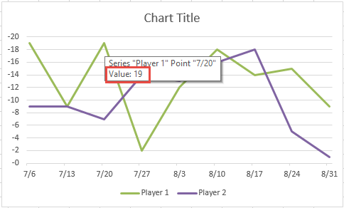
How To Make An Excel Chart Go Up With Negative Values Excel Dashboard Templates
Excel Waterfall Charts Bridge Charts Peltier Tech

How To Move Chart X Axis Below Negative Values Zero Bottom In Excel
Negative Values Not Displaying In Y Axis Or Data Labels On Chart


Moving The Axis Labels When A Powerpoint Chart Graph Has Both Positive And Negative Values
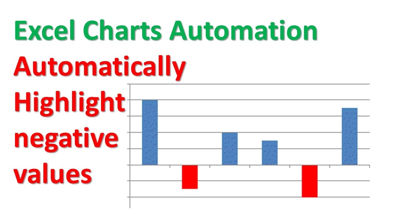
Excel Charts Automatically Highlight Negative Values Youtube

How To Plot Positive And Negative Values On Both Sides Of The Axis In Excel Super User

Best Excel Tutorial Chart With Negative Values
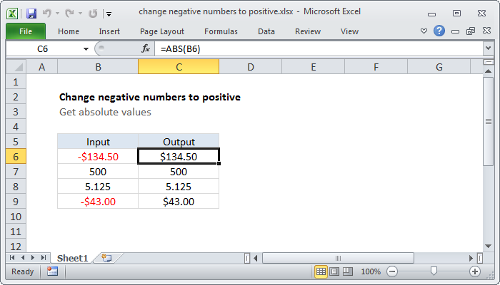
Excel Formula Change Negative Numbers To Positive Exceljet
Excel Waterfall Charts Bridge Charts Peltier Tech
Visually Display Composite Data How To Create An Excel Waterfall Chart Pryor Learning Solutions
How To Make An Excel Chart Go Up With Negative Values Excel Dashboard Templates
How To Make An Excel Chart Go Up With Negative Values Excel Dashboard Templates
How To Make An Excel Chart Go Up With Negative Values Excel Dashboard Templates
How To Set Different Colors To Separate Positive And Negative Number In Bar Chart Free Excel Tutorial

Positive Negative Bar Chart Beat Excel
Advanced Excel Waterfall Chart Tutorialspoint

How To Separate Colors For Positive And Negative Bars In Column Bar Chart